Algorithm Analysis
How fast is a program?1 If the (time) efficiency is our major concern, then we have to ask this question regularly.
A hands-on method
A straightforward way is to measure the elapsing time. In the following, we will use a tiny program (Fibonacci.java and fibonacci.py) to compute the nth fibonacci number.
Java
In Java, there are many APIs available in terms of time/date, including System.currentTimeMillis(), Instant.now. You can use either of the following method2 to compute the elapsing time in milliseconds:
long start = System.currentTimeMillis();
// your program runs
long end = System.currentTimeMillis();
long elapse = end - start;
long start = Instant.now().toEpochMilli();
// your program runs
long end = Instant.now().toEpochMilli();
long elapse = end - start;
Instant start = Instant.now();
// your programs runs
Instant end = Instant.now();
long elapse = Duration.between(start, end).toMillis();
A more robust and comprehensive approach in Java is to use JMH, and the usage of it is out of the scope of this book.
Python
In Python, several modules can be used to deal with time/date, including time, datetime. But note that time.time() returns a float number representing the current time in seconds since the Epoch. You can use either of the following code to compute the elapsing time in milliseconds:
start = int(round(time.time() * 1000))
# your program runs
end = int(round(time.time() * 1000))
elapse = end - start
start = datetime.datetime.now()
# your program runs
end = datetime.datetime.now()
elapse = int(round((end - start).total_seconds() * 1000))
Generally, to avoid the variability of the running time, we usually run the program for several times and then take the average. Luckily, the built-in timeit makes it simple.
Visualize the efficiency
Sometimes, we would like to visualize the quantitative measurements of the running time of our programs. A common qualitative observation about most programs is that there is a problem size
that characterizes the difficulty of the computational task. For example, fibonacci(30) will definitely coast more time than fibonacci(3). Here the parameter (i.e., 3 and 30) can be seen as the problem size.
A simple way is to save (size, time) per line in a file (FibTime.java and fib_time.py), and then to visualize results using tools like gnuplot, ggplot2 in R, Matplotlib in Python, and Plotly Express in Python.
Many people tend to plot the data from the memory directly, but plotting the data from a file is more common in practice. Therefore, we deliberately separate the data computing and plotting in this book.
Here I use the Python version as the example:
if __name__ == '__main__':
    ns = [20, 21, 22, 23, 24, 25, 26, 27, 28, 29, 30]
    with open('fib_python.txt', 'w') as f:
        for n in ns:
            start = int(round(time.time() * 1000))
            fibonacci(n)
            end = int(round(time.time() * 1000))
            f.write(f'{n}   {end - start}\n')
Note that here the problem size starts from 20, because the time is near to 0 when the problem size is less than 20.
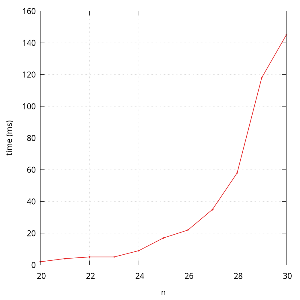
According to the observation3, some students may quickly make an insightful hypothesize that the running time is at an exponential growth, and I will analyze it through a mathematical model soon. By the way, the Java version of Fibonacci is much faster than the Python version.
Mathematical models
D.E. Knuth postulated that, despite all the complicating factors in understanding the running times of our programs, it is possible, in principle, to build a mathematical model to describe the running time of any program. Knuth’s basic insight is simple: the total running time of a program is determined by two primary factors:
- The cost of executing each statement
- The frequency of execution of each statement
The former is a property of the computer and the language itself, and the second one is a property of the program and the input. The primary challenge is to determine the frequency of execution of the statements. Here are some examples:
def foo(n):
    for i in range(n):
        print(i)
The frequency of the inner statement of this function is n.
Sometimes, frequency analysis can lead to complicated and lengthy mathematical expressions. Consider the two-sum problem, and the following is a naive solution:
class Solution:
    def two_sum(self, nums, target):
        for i, v in enumerate(nums):
            for j in range(i + 1, len(nums)):
                if v + nums[j] == target:
                    return [i, j]
        return []
The frequency of the inner comparison test statement of this function is (n-1) + (n-2) + ... + 1 in the worst case:
\[ \frac{n \times (n-1)}{2} = \frac{n^2 - n}{2} \]
Curious readers can try to implement a faster algorithm for this problem4. Note that here I put emphasis on the worst case, because if you are lucky enough, the sum of the first and second item equals target, then the frequency in the best case is only 1.
As for the notation \(\frac{n^2 - n}{2}\), we can know that it is the \(\frac{n^2}{2}\) that plays a major rule in terms of the growth, so we can say \(\frac{n^2}{2}\) approximates to \(\frac{n^2 - n}{2}\). In addition, when it comes to the order of growth, the constant here (i.e., 1/2) is also insignificant. The following shows some typical approximations:
| Function | Approximation | Order of growth |
|---|---|---|
| \(N^3/6 - N^2/2 + N/3\) | \(N^3/6\) | \(N^3\) |
| \(N^2/2 - N/2\) | \(N^2/2\) | \(N^2\) |
| \(lg{N} + 1\) | \(lg{N}\) | \(lg{N}\) |
| 3 | 3 | 1 |
The order of growth in the worst case can be also described by the big O notation, e.g., \(O(n^3)\). The following shows some commonly encountered time complexity using the big O notation:
| Description | Time complexity |
|---|---|
| constant | \(O(1)\) |
| logarithmic | \(O(log{N})\) |
| linear | \(O(N)\) |
| linearithmic | \(O(N\log{N})\) |
| quadratic | \(O(N^2)\) |
| cubic | \(O(N^3)\) |
| exponential | \(O(2^N\)) |
For example, we can say
- the complexity of
foo()is \(O(N)\) - the complexity of
two_sum()is \(O(N^2)\)
Case study: Fibonacci
Based on the observation, we make an insightful hypothesize that the running time of recursive implementation fibonacci is at an exponential growth.
According to the code, we know that in order to computer fibonacci(n), it is required to compute fibonacci(n - 1) and fibonacci(n - 2). If we use \( T(n) \) to denote the time used to compute fibonacci(n), then we have:
\[T(n) = T(n-1) + T(n-2) + O(1)\]
The \(O(1)\) here means the addition operation. You can prove that \(T(n) = O(2^n)\)5, and the visualization plotting also validates this theoretical result.
1 Another important question is "Why does my program run out of memory?", which cares about the space efficiency.
2 See more at https://stackoverflow.com/questions/58705657/.
3 This figure is drawn by gnuplot and the code can be found at lines.gp.
4 It is possible to design faster algorithms with \( O(N\log{N}) \) and even with \( O(N) \).
5 See more at https://www.geeksforgeeks.org/time-complexity-recursive-fibonacci-program/.